How to Calculate IRR in Excel: IRR, XIRR, and MIRR Functions (2026)
IRR in Excel uses three functions depending on cash flow timing. When to use =IRR, =XIRR, and =MIRR, with syntax, worked examples, and #NUM! fixes.
Most people learn one Excel IRR function and assume it is the right one for every situation. It usually is not. Excel has three separate functions for IRR calculations, and using the wrong one for irregular cash flow timing or deals with large interim distributions produces a number that looks precise but is actually wrong.
The IRR Calculator handles this automatically without a spreadsheet. For analysts who need to build or audit their own models in Excel, this guide covers the exact syntax and correct use case for each function, the input errors that come up most often, and how to recover from a #NUM! result when the solver fails.
Excel's Three IRR Functions and When to Use Each
Excel provides =IRR(), =XIRR(), and =MIRR(). They solve related but different problems. Choosing the wrong function for a given investment structure is one of the most common modeling errors in real estate and private equity analysis.
The Financial Calculator IRR Guide covers IRR on physical devices like the HP 12C and BA II Plus. This post focuses entirely on Excel.
The table below shows which function fits which situation.
| Function | Cash Flow Timing | What It Returns |
|---|---|---|
| =IRR(values) | Equal intervals (annual, monthly, etc.) | Standard annualized IRR |
| =XIRR(values, dates) | Irregular calendar dates | True annualized IRR |
| =MIRR(values, finance_rate, reinvest_rate) | Equal intervals | Modified IRR (realistic reinvestment rate) |
The most important choice is between =IRR() and =XIRR(). For any real deal where cash flows occur on specific dates rather than perfectly at year-end, =XIRR() is the more accurate function. Most analysts default to =IRR() and accept the approximation error; for long holds with irregular timing, that error can shift the result by 1-2 percentage points.
=IRR(): The Standard Formula for Annual Cash Flows
Syntax:
=IRR(values, [guess])
- values: a range of cells starting with the initial investment as a negative number, followed by each period's cash flow in order
- guess (optional): a starting estimate for Excel's iteration. Defaults to 10% if omitted. Useful when the result is unusual or the solver struggles to converge.
Setup example: a 5-year investment
Structure the spreadsheet with the initial outflow first and each year's cash flow after it:
A1: -500000    (Year 0 initial investment, must be negative)
A2:  80000     (Year 1 cash flow)
A3:  90000     (Year 2)
A4:  95000     (Year 3)
A5: 100000     (Year 4)
A6: 750000     (Year 5 including sale proceeds)

B1: =IRR(A1:A6)
Result: 18.41%
Two rules that trip people up more than any other:
The initial investment must be negative. If you enter it as positive, Excel treats year 0 as an inflow and solves for a different problem. The result will be wrong and may not produce an error. Always use a negative sign or a formula like =-B3 to link to a positive input cell.
Blank cells are treated as zeros. If year 3 has no cash flow, enter 0 in that cell, do not leave it blank. Excel treats blank cells as not part of the series, shifting the timing of every subsequent cash flow and producing a wrong result without any warning.
The optional guess parameter: Excel's IRR solver starts at 10% and iterates using Newton-Raphson. For most standard investments this converges instantly. For unusual cash flow patterns (very high or very low returns, long series), supplying a guess closer to the expected result helps convergence: =IRR(A1:A6, 0.25) for a deal expected to return around 25%.
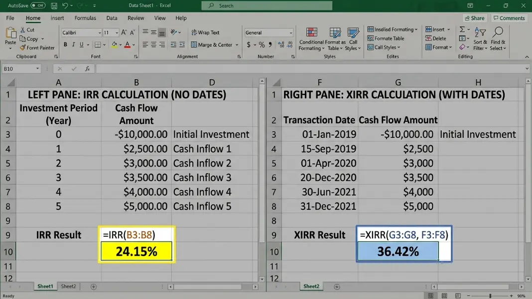
=XIRR(): Why You Should Use It for Most Real Deals
Syntax:
=XIRR(values, dates, [guess])
=XIRR() takes a column of specific calendar dates alongside the cash flows and calculates the true annualized rate based on the actual time between each flow. For any investment where cash flows do not fall at exact year-end intervals, =XIRR() is the more accurate choice.
When =IRR() produces the wrong answer: Suppose you close on a property on March 15 and sell it on November 1 three years later. =IRR() treats year 3 as exactly 36 months after year 0. =XIRR() counts the actual 32.5 months and adjusts the annualized rate accordingly. For longer holds, this timing difference compounds and can shift the result by 1-2 percentage points.
Setup example with actual dates:
A1: -500000    B1: 3/15/2023   (closing date)
A2:   3200     B2: 4/1/2023    (first month's net rent)
A3:   3200     B3: 5/1/2023
...
A38: 650000    B38: 11/1/2026  (sale proceeds + final month)

C1: =XIRR(A1:A38, B1:B38)
The dates in column B must be in a format Excel recognizes as dates, not text. If =XIRR() returns #VALUE!, check whether the date cells are formatted as dates. A quick test: click on a date cell. If the formula bar shows a raw number (like 45123), the dates are stored as numbers and will work. If it shows text (like "3/15/2023" left-aligned), they are stored as text and must be converted.
Monthly cash flows with XIRR: Unlike =IRR(), =XIRR() always returns an annualized rate regardless of how frequently cash flows occur. Entering monthly rents with actual monthly dates gives you an annual IRR directly, with no manual annualizing step.
=MIRR(): Fixing the Reinvestment Rate Problem
Syntax:
=MIRR(values, finance_rate, reinvest_rate)
Standard IRR has a known flaw: it assumes every interim cash flow is reinvested at the IRR rate itself. A deal with a 20% IRR assumes you can put every distribution back to work at 20% indefinitely. For most investors, that assumption is too optimistic, which makes standard IRR an inflated estimate of the investment's true performance.
=MIRR() fixes this by letting you specify two rates separately:
- finance_rate: your cost of capital for negative cash flows (borrowing rate, typically 6-9% in 2026)
- reinvest_rate: the realistic rate at which you reinvest positive cash flows (typically 5-8%, reflecting expected market returns)
Example: same 5-year investment with realistic rates
A1: -500000
A2:  80000
A3:  90000
A4:  95000
A5: 100000
A6: 750000

B1: =MIRR(A1:A6, 7%, 5%)
Result: 15.82%

Compare: =IRR(A1:A6) = 18.41%
The gap between =IRR() (18.41%) and =MIRR() (15.82%) is the cost of the unrealistic reinvestment assumption. If your hurdle rate is 14%, the deal clears on both metrics. If your hurdle is 16%, standard IRR says accept while MIRR says reject, and MIRR is the more honest answer.
For most real estate analysis, =MIRR() with 6-7% finance rate and 4-6% reinvestment rate gives a more conservative and defensible number. The IRR Formula Guide covers the mathematical relationship between IRR and MIRR in detail, including how the reinvestment assumption affects the result as the standard IRR increases.
One important limitation: =MIRR() uses equal-interval cash flows like =IRR(). There is no XMIRR equivalent in Excel. For deals with irregular timing, calculate standard XIRR and then apply a manual MIRR adjustment, or note the limitation when presenting results.
Why Excel Returns #NUM! and How to Fix It
#NUM! is Excel's indication that the IRR solver failed to find a solution. Three distinct problems produce this error.
Problem 1: No sign change in the values
=IRR() requires at least one negative and one positive cash flow. If the initial investment is entered as positive (a common mistake), or if a deal produces no recovery of any capital, no mathematical IRR solution exists.
Fix: confirm the first value in the range is negative. If you link to an input cell that stores the investment as a positive number, use =-B3 to flip the sign in the cash flow range.
Problem 2: Solver cannot converge from the default starting guess
The default 10% guess is too far from the true solution for investments with unusual return profiles: very short holds with extreme returns, very long series with slow compounding, or real estate workouts with initial negative cash flows from capital improvements.
Fix: supply a different guess. =IRR(A1:A10, 0.30) for a high-return estimate. =IRR(A1:A10, -0.10) for an investment expected to produce a partial loss. Try several guesses: 0.05, 0.15, 0.30. If none converge, the investment may have a multiple IRR problem.
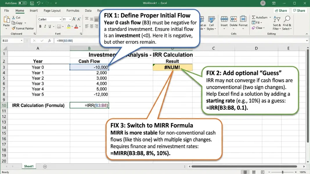
Problem 3: Multiple sign changes (multiple IRR problem)
When cash flows alternate between positive and negative more than once, the IRR equation can have multiple mathematically valid roots. Excel returns one value (which one depends on the starting guess) or returns #NUM! if the iteration diverges. Neither result is reliable.
Fix: use =MIRR() instead. =MIRR() always produces a unique answer regardless of how many sign changes exist in the cash flow series.
Once you have a calculated IRR, the What Is a Good IRR Guide puts the number in context: what the benchmarks are by asset class and holding period, and when a high IRR is not telling the full story about wealth creation.
Use =IRR(values) for cash flows at equal time intervals. Enter the initial investment as a negative number in the first cell of the values range, then each period's cash flow in sequence. The function returns the annualized IRR. For cash flows on specific calendar dates, use =XIRR(values, dates) instead. For a version that uses a realistic reinvestment rate rather than the default assumption, use =MIRR(values, finance_rate, reinvest_rate).
=IRR() assumes equal time intervals between every cash flow. =XIRR() takes actual calendar dates for each cash flow and calculates the true annualized return based on exact time differences. For deals where cash flows occur on specific dates rather than at exact year-end intervals, =XIRR() is more accurate. =IRR() is acceptable for simplified annual models. =XIRR() is the right choice for any real investment with specific transaction dates, including monthly rent collection or mid-year closings.
Excel returns #NUM! when the IRR solver fails to find a solution. The three main causes are: the values range contains no sign change (all positive or all negative), the starting guess is too far from the true answer (fix with a custom guess like =IRR(A1:A10, 0.30)), or the cash flows change sign more than once (the multiple IRR problem). For multiple sign changes, switch from =IRR() to =MIRR(), which always returns a unique solution.
=MIRR(values, finance_rate, reinvest_rate) calculates Modified IRR, which separates the borrowing rate for negative flows from the reinvestment rate for positive flows. Standard =IRR() assumes all interim distributions are reinvested at the IRR rate itself, which overstates performance when the IRR is well above market rates. Use =MIRR() when presenting conservative return estimates to investors, comparing deals with large interim cash flows, or whenever your standard IRR significantly exceeds realistic reinvestment opportunities.
Yes. =IRR() treats whatever interval you enter as one period. Monthly cash flows entered in =IRR() return a monthly rate, not an annual one. To annualize it: =(1 + monthly_IRR)^12 - 1. For annual cash flows, =IRR() returns the annual rate directly. =XIRR() sidesteps this issue entirely by taking actual calendar dates and always returning an annualized rate, regardless of how frequently the cash flows occur.
Use =XIRR() with actual calendar dates. Enter the sale date in the dates column and the exit proceeds in the corresponding values cell. =IRR() will mistime the exit if it does not fall at an exact year-end. =XIRR() handles any partial-year hold accurately. If you must use =IRR(), a rough approximation treats the final period as fractional by prorating the last year's cash flow, but =XIRR() is the correct approach for real deal analysis.
Written by
Hassaan Rasheed
Web Developer & Content Researcher
Hassaan builds calculators and writes research-backed guides on finance, math, payroll, and construction topics. Every number in his articles is sourced from official data and worked through by hand.
View LinkedIn Profile