Partial Derivative Calculator: How Partial Differentiation Works (2026)

Partial derivatives measure how a multivariable function changes in one direction while all others are fixed. Rules, worked examples, gradient, and real applications.

A partial derivative measures how a function changes when one variable increases while every other variable is held fixed. If f(x, y) = x^2 + 3xy + y^3, the partial derivative with respect to x tells you the rate of change in the x direction while y is frozen at its current value. The partial derivative with respect to y gives you the same information in the y direction while x is frozen.

This operation is the foundation for optimization in multiple dimensions, gradient descent in machine learning, and partial differential equations in physics. Use the Partial Derivative Calculator for step-by-step results. This guide covers how to calculate partial derivatives, second-order and mixed derivatives, the gradient vector, and how these concepts appear in real problems.

How to Calculate a Partial Derivative

The notation for partial derivatives uses the rounded symbol ∂ instead of the straight d of ordinary differentiation. ∂f/∂x means: differentiate f with respect to x, treating every other variable as a constant.

The rules are identical to single-variable calculus. Power rule, product rule, quotient rule, chain rule, all apply exactly as usual. The only change is interpretation: any variable you are not differentiating with respect to is treated as a fixed number.

Worked example 1:

f(x, y) = 3x^2 y + 2xy^3 - 5y^2

To find ∂f/∂x: treat y as a constant throughout.

• 3x^2 y: y is a constant multiplier, so differentiate x^2 using the power rule → 6xy
• 2xy^3: y^3 is a constant, derivative of x is 1 → 2y^3
• -5y^2: contains no x, so derivative = 0

∂f/∂x = 6xy + 2y^3

To find ∂f/∂y: treat x as a constant throughout.

• 3x^2 y: x^2 is a constant, derivative of y is 1 → 3x^2
• 2xy^3: x is a constant, power rule on y^3 → 6xy^2
• -5y^2: power rule on y^2 → -10y

∂f/∂y = 3x^2 + 6xy^2 - 10y

Worked example 2 (with trigonometric and exponential terms):

g(x, y) = x^2 sin(y) + e^x cos(y)

∂g/∂x:

• x^2 sin(y): sin(y) is a constant, differentiate x^2 → 2x sin(y)
• e^x cos(y): cos(y) is a constant, derivative of e^x is e^x → e^x cos(y)

∂g/∂x = 2x sin(y) + e^x cos(y)

∂g/∂y:

• x^2 sin(y): x^2 is a constant, derivative of sin(y) is cos(y) → x^2 cos(y)
• e^x cos(y): e^x is a constant, derivative of cos(y) is -sin(y) → -e^x sin(y)

∂g/∂y = x^2 cos(y) - e^x sin(y)

Second-Order and Mixed Partial Derivatives

Second-order partial derivatives differentiate twice. The notation distinguishes between differentiating the same variable twice and differentiating two different variables.

• ∂²f/∂x² (also written fxx): differentiate with respect to x, then again with respect to x
• ∂²f/∂y² (also written fyy): differentiate with respect to y, then again with respect to y
• ∂²f/∂y∂x (also written fxy): differentiate with respect to x first, then with respect to y
• ∂²f/∂x∂y (also written fyx): differentiate with respect to y first, then with respect to x

Clairaut's theorem: For functions whose second-order mixed partials are continuous, the order of differentiation does not matter: ∂²f/∂x∂y = ∂²f/∂y∂x. You can differentiate in whichever order is easier.

Example using f(x, y) = 3x^2 y + 2xy^3:

From earlier: ∂f/∂x = 6xy + 2y^3 and ∂f/∂y = 3x^2 + 6xy^2

Second-order partials:

∂²f/∂x^2 = ∂/∂x(6xy + 2y^3) = 6y

∂²f/∂y^2 = ∂/∂y(3x^2 + 6xy^2) = 12xy

Mixed partial (differentiate fx with respect to y): ∂²f/∂y∂x = ∂/∂y(6xy + 2y^3) = 6x + 6y^2

Mixed partial (differentiate fy with respect to x): ∂²f/∂x∂y = ∂/∂x(3x^2 + 6xy^2) = 6x + 6y^2

Both mixed partials equal 6x + 6y^2, confirming Clairaut's theorem.

The Gradient Vector

The gradient collects all first-order partial derivatives into a single vector. It is written ∇f (called "del f" or "grad f").

For f(x, y): ∇f = (∂f/∂x, ∂f/∂y)

For f(x, y, z): ∇f = (∂f/∂x, ∂f/∂y, ∂f/∂z)

What the gradient tells you:

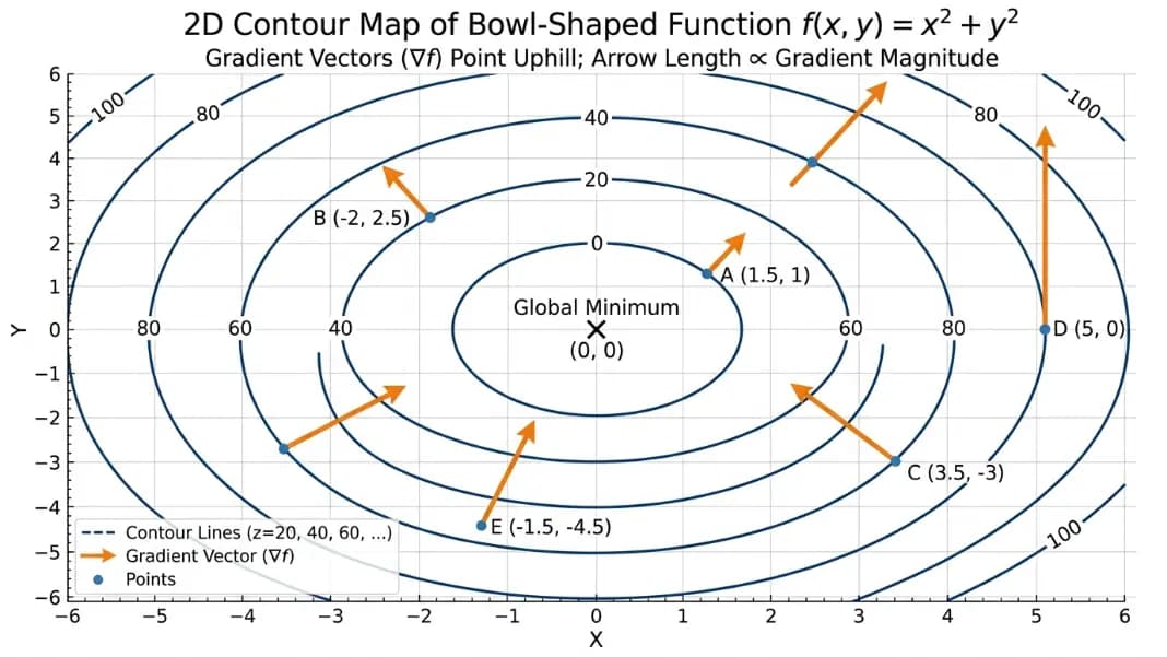
The gradient vector points in the direction of steepest increase of f at any given point. Its magnitude is the rate of increase in that direction. The negative gradient (-∇f) points in the direction of steepest decrease.

Example:

f(x, y) = x^2 + y^2

∂f/∂x = 2x, ∂f/∂y = 2y

At the point (3, 4): ∇f = (6, 8). The direction of steepest ascent from (3, 4) is the vector (6, 8). The magnitude (rate of increase in that direction) = sqrt(36 + 64) = sqrt(100) = 10.

Moving one unit in the direction (6/10, 8/10) from (3, 4) increases f by approximately 10 per unit of distance.

Gradient descent in machine learning:

In neural network training, the loss function L depends on millions of parameters (weights). To minimize L, training computes the gradient ∇L with respect to all weights simultaneously, then updates each weight by subtracting a small fraction of its partial derivative:

w_new = w_old - learning_rate x (∂L/∂w)

This single step, applied repeatedly, moves the parameters toward lower loss. The chain rule for partial derivatives makes it possible to compute ∂L/∂w for every weight efficiently, layer by layer from output to input. That process is backpropagation.

Finding Critical Points Using Partial Derivatives

To find local maxima, minima, or saddle points of f(x, y), set all first-order partial derivatives equal to zero and solve the resulting system.

Procedure:

1. Compute ∂f/∂x and ∂f/∂y
2. Set both equal to zero and solve for (x, y)
3. Classify each critical point using the second derivative test

Second derivative test:

Compute D = (∂²f/∂x^2)(∂²f/∂y^2) - (∂²f/∂x∂y)^2

• D > 0 and ∂²f/∂x^2 > 0: local minimum
• D > 0 and ∂²f/∂x^2 < 0: local maximum
• D < 0: saddle point (neither min nor max)
• D = 0: the test gives no information

Worked example:

f(x, y) = x^2 - 4x + y^2 - 6y + 15

∂f/∂x = 2x - 4 = 0 → x = 2

∂f/∂y = 2y - 6 = 0 → y = 3

Critical point: (2, 3)

∂²f/∂x^2 = 2, ∂²f/∂y^2 = 2, ∂²f/∂x∂y = 0

D = (2)(2) - (0)^2 = 4 > 0, and ∂²f/∂x^2 = 2 > 0

(2, 3) is a local minimum. f(2, 3) = 4 - 8 + 9 - 18 + 15 = 2

Real Applications of Partial Derivatives

Heat equation: ∂u/∂t = k x ∂²u/∂x^2 describes how temperature u spreads through a material over time. The partial with respect to time on the left; the second partial with respect to position on the right. Every numerical weather model and thermal simulation solves variations of this equation.

Economics: If profit π depends on labor L and capital K, then ∂π/∂L is the marginal product of labor: the change in profit from hiring one more worker. Setting both ∂π/∂L and ∂π/∂K to zero finds the input combination that maximizes profit. This is standard constrained optimization in microeconomics.

Options pricing (the Greeks): Delta = ∂V/∂S is the partial derivative of an option's value with respect to the underlying stock price. Gamma = ∂²V/∂S^2 is the second partial. Theta, Vega, and Rho are all partial derivatives of option value with respect to other input variables (time, volatility, interest rate).

Fluid mechanics: The Navier-Stokes equations, which govern how fluids flow, are a system of partial differential equations involving partial derivatives of velocity with respect to position and time. Solving them numerically is the core challenge of computational fluid dynamics.